Fastai Lesson 2
Deploying a trained computer vision model
Disclaimer:
In the unlikely event that the person reading this is not me, please make sure to check out the actual course “Deep Learning for Coders” over at course.fast.ai. These summaries are written with an audience of one - me - in mind, so proceed with caution.
Deploying a trained computer vision model with fastai
After Lesson 1 provided a general introduction to the fastai library and the steps involved in training a deep learning model, the second lesson goes on to explain how to use the fine-tuned model in a production environment. The lessons covers numerous topics beyond this but in this blog, I take the liberty of limiting my notes on the parts most relevant to me, personally.
Bing image search
As established in the first lesson, the intitial step in training a machine learning application is the acquisition and preparation of data. Since the example is a computer vision model, Jeremy uses this opportunity to showcase the Bing image search functionality within the fastai library.
The steps below outline the required actions to load images to disk based on a search query:
- sign up to Azure Cognitive Services
- extract your API key
- use fastai image search functionality
I will not go into the actual steps involved in setting up Azure Cognitive Services - google is your friend! The interesting parts for this article are around the use of the Bing image search in fastai.
Quick example of using search_images_bing to load a single image:
key = '[Replace with actual API key]'

results = search_images_bing(key, 'grizzly bear')
ims = results.attrgot('content_url')

dest = 'images/grizzly.jpg'
download_url(ims[0], dest)  # returns 150 urls by default

image = Image.open(dest)
image.to_thumb(128,128)
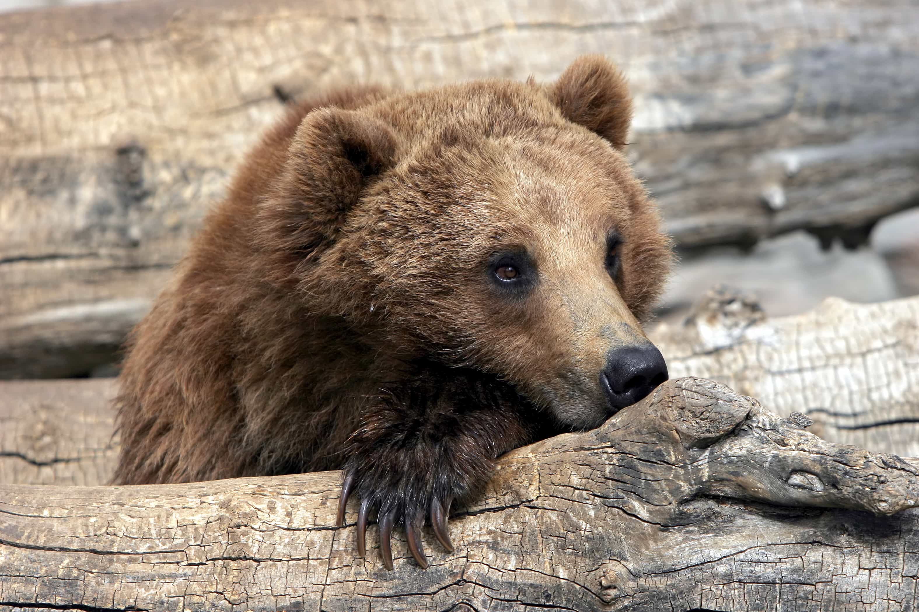
Running this with your personal Bing Search API key should yield something like the below output:

This image data can be used to train a model which can distinguish between grizzly bears, black bears and teddy bears (the example use case of the course):
bear_types = 'grizzly', 'black'
path = Path('bears')

if not path.exists():
   path.mkdir()
   for bt in bear_types:
      dest = (path/bt)
      dest.mkdir(exist_ok=True)
      results = search_images_bing(key, f'{bt} bear')
      download_images(dest, urls=results.attrgot('content_url'))

file_names = get_image_files(path)
To check whether all of the downloaded files are actually images, fastai offers a function called
verify_images, which returns a list of failed images. To remove those, you can call
Path.unlinkin order to delete those files:
failed = verify_images(file_names)
failed.map(Path.unlink)
Note that map in the above example is also a fastai method.
The DataBlock API
As an example computer vision application, I want to train a classifier that can differentiate between images of grizzly bears, black bears and my dog, Emil (pictured below).

So as a first step, we need to prepare the training and validation sets of labeled images.
The first lesson utilized a factory method to prepare the DataLoaders class. While this is highly efficient, fastai also provides a more flexible approach to get from data to DataLoaders - the DataBlock API:
bears = DataBlock(blocks=(ImageBlock, CategoryBlock), # inputs are images, labels are categories
                  get_items=get_image_files,
                  splitter=RandomSplitter(valid_pct=0.3, seed=42),  # random split into train, valid
                  get_y=parent_label,  # name of the containing folder acts as label
                  item_tfms=Resize(128))

dls = bears.dataloaders(path)  # create DataLoaders instance from DataBlock instance
Once the data is prepated in the form of a DataLoaders instance, the model can be trained as discussed in the first lesson:
learn = cnn_learner(dls, resnet18, metrics=error_rate)
learn.fine_tune(4)
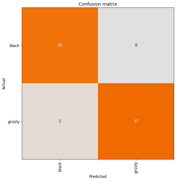
Going a step further than the first lesson, let’s examine the result of the training run in a bit more detail:
interp = ClassificationInterpretation.from_learner(learn)
interp.plot_confusion_matrix()
This yields the following confusion matrix:

This is obviously a classic visualization of the performance of a machine learning model, however,
Jeremy also argues for its merit in the use of analyzing the underlying dataset. As the cross-industry standard for data mining (Shearer, 2000) also indicates, data preparation and modelling are not strictly sequential and require a certain amount of back and forth between the steps. The lesson shows, that the analysis of the data does not only inform the modelling step but also the other way around - the model shows idiosyncrasies in the data that might otherwise go undiscovered.
A very useful function for using the trained model to analyze the underlying data set is the
plot_top_losses function:
interp.plot_top_losses(5, nrows=1)
The plot_top_losses returns the specified number of images with the highest loss. The below image
shows the output:

The output allows the data scientist to discover underlying issues with the data, such as incorrectly labeled images, or weaknesses of the current model, like uncommen angles or poses that should be included more often in training. In this case none of the top losses where incorrect predictions, however it looks like some images of black bears were incorrectly labeled as grizzlies.
Deploying a deep learning model to production
The fastai library easily allows for exporting trained models as .pkl files. Similarly, saved
learners can be imported from disk using the load_learner function.
learn.export()  # saves model as 'export.pkl'
learn = load_learner(path/'export.pkl')  # imports existing learner from disk
And that’s it! The combination of export and load_learner allows you to move your trained model to a
server and use it in production.
References:
- Shearer, C. (2000). The CRISP-DM Model: The New Blueprint for Data Mining. Journal of Data Warehousing, 5(4).